CLIPC: Constructing Europe's Climate Information Portal

Use case finding the geographic sensitivity of vegetation growth to temperature in Europe

Starting point

In the course of a long drive during early spring, an impact researcher becomes puzzled as to why vegetation growth in some geographic locations in central Europe appears to be well underway, while in other locations it has not even started, even though the ambient temperatures in all locations appear to be the same. He sets out to determine:

• The geographic sensitivitysensitivity
  The degree to which a system or species is affected, either adversely or beneficially, by climate variability or change. The effect may be direct (e.g., a change in crop yield in response to a change in the mean, range or variability of temperature) or indirect (e.g., damages caused by an increase in the frequency of coastal flooding due to sea-level rise). of vegetation growth to temperature in Europe.

For the purposes of evaluating the response function of vegetation growth to temperature the impact researcher conceives a simple theoretical framework shown in the figure below (top) as well as the analytical formulation and indicators required (bottom).

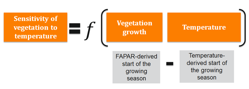
He knows that the start of the growing season is a good indicator of when the conditions are suitable for vegetation to develop. Even better, this indicator seems to be available for two distinct methodologies, namely, one that only makes use of meteorological observations from weather stations (i.e. daily average temperature) and a second one that uses information on vegetation growth measured by satellite (i.e. the so-called Fraction of Absorbed Photosynthetically Active Radiation, or FAPAR). A difference, or time-lag, between the dates for the start of the growing season from these two approaches, indicate the sensitivity of vegetation growth to temperature across Europe.

 Basic approach

The analysis comprises three tasks:

• Determining FAPAR-derived start of the growing season.
• Determining temperature-derived start of the growing season.
• Determining the time lag between the two.

Basic indicators

• Start of the Growing Season (temperature derived)
• Start of the Growing Season (FAPAR derived)

CLIP-C tools featured

Map viewer, Combine tool

Contact person

Niall McCormick, JRC.

Analytical steps in detail

1. Select the ecosystem theme on the left side of the combine tool.
   
   
2. Load indicator ‘start of the growing season’.
   
   
3. Select the following dataset: SGS pheno JRC 1.0 EC-JRC FAPAR JRC yr 19980101-20111231 1998-2011
   
   
4. Select the 2010 time stamp
   
   
5. Load indicator ‘start of the growing season’ in the right side of the combine tool
   
   
6. Select the following dataset: sgs induce-1-0-0 EC-JRC MARS-AGRI4CAST yr 19750101-20151231 1975-2015
   
   
7. Select the 1991-2010 time period
   
   
8. Select “none” in the normalization box
   
   
9. Select subtract in the process box
   
   
10. Name the output as “gst-change.nc”
    
    
11. Hit execute

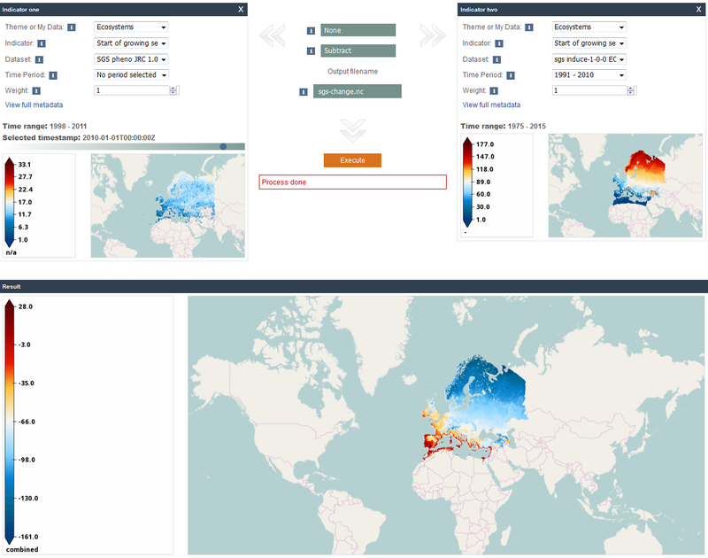
The result shows, for a given year, the time-lag between the start of the growing season, as defined by the period warm enough for vegetation growth (i.e. average daily temperatures above 5°C), and the actual start of vegetation growth, as measured by satellite. Differences in the time-lag for different geographic locations highlight variations in temperature sensitivity of spring vegetation growth across Europe.